Author: Anya Sinha

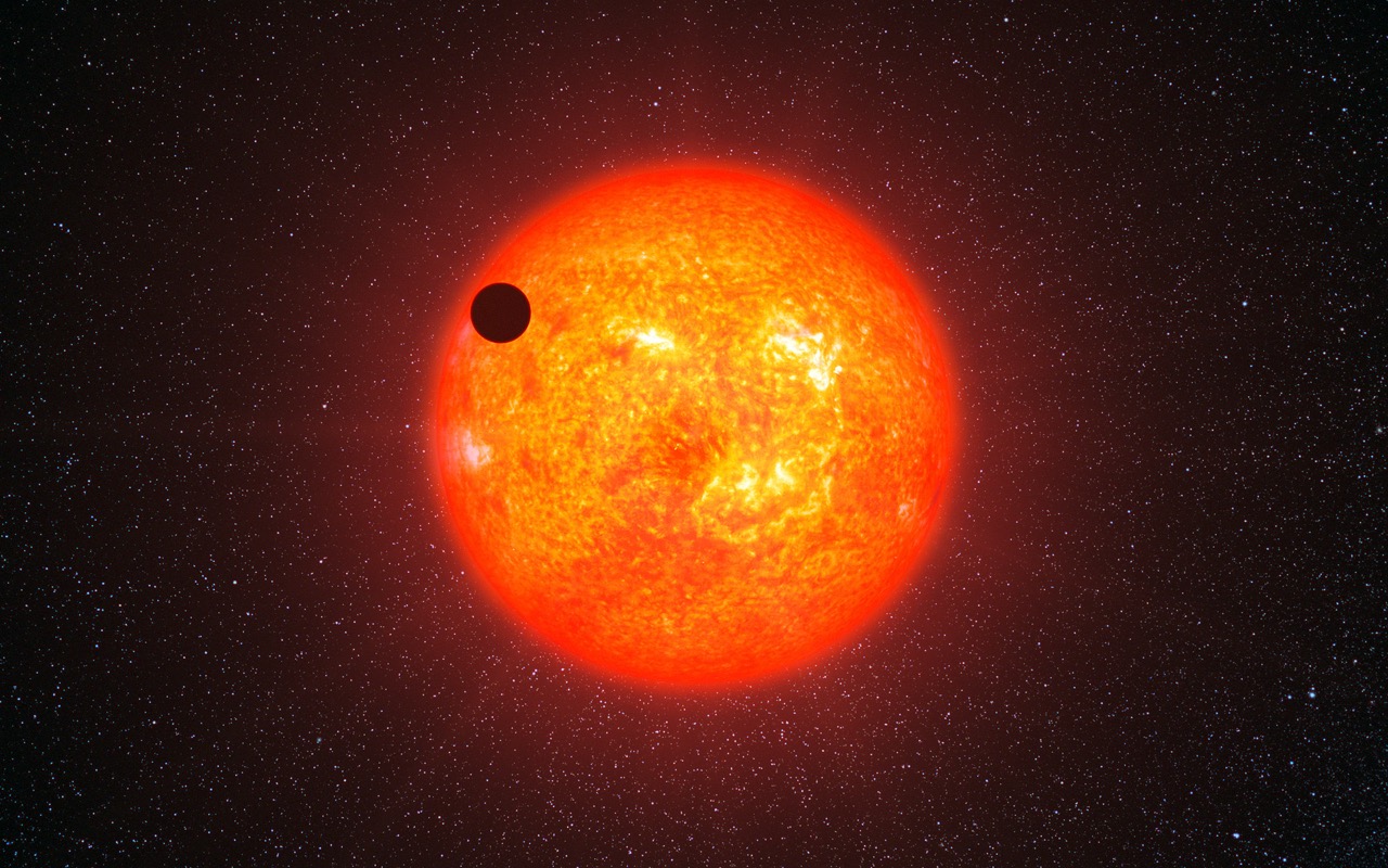
Photo by ESO/L. Calçada from Wikimedia Commons, 1 December 2010

Figure 1: Picture of an exoplanet in front of a star

How do you find something you cannot see? You look for what it leaves behind. After an Edinburgh shower, you may not have seen the rain fall, but the wet pavements give it away. Finding exoplanets works the same way. Most exoplanets are too faint and too close to the stars they orbit to photograph directly. These stars are known as host stars, and exoplanets are often lost in their bright glare. 

An exoplanet is a planet orbiting a star beyond our solar system. Usually, the stars of these planets are billions of times brighter than the planets themselves. Thus, trying to photograph the planet directly is like trying to spot a firefly next to a powerful flashlight: the much brighter light can overwhelm the firefly’s faint glow. Rather than looking for the planet itself, astronomers search for the subtle effects it has on the light of its host star. One of the most successful methods is called the transit method.

A transit occurs when a planet passes between its host star and the observer. As the planet crosses in front of the star, it blocks a small amount of the star’s light. The star therefore appears to become slightly dimmer. By measuring the star’s brightness over time, astronomers create a graph known as a light curve, which typically looks like this:

Photo by NASA Ames from Flickr

Figure 2: General shape for a light curve

The dip in the graph represents the transit. Its depth depends approximately on the squared ratio of the planet’s area to the star’s area. This is shown in the formula below, where $R_p$ is the planet’s radius, $R_*$ is the star’s radius, $F$ stands for the star’s normal flux (brightness), and $ΔF$ is the brightness decrease during the transit. Thus, $\frac{ΔF}{F}$ is the fractional decrease in the star’s brightness. 

A larger planet blocks a larger fraction of the star’s light and therefore produces a deeper dip in brightness. For comparison, a Jupiter-sized planet crossing a Sun-sized star can block roughly 1% of its light, while an Earth-sized planet produces a dip closer to 0.01%. While both represent tiny changes in brightness levels, modern telescopes are advanced enough to measure them. In fact, the purpose of NASA’s Kepler mission was to monitor thousands of stars to search for these small changes in brightness and, hopefully, discover new exoplanets. 

However, a single dip is not enough to confirm the existence of a planet. Small fluctuations or errors in the telescope’s detector, known as instrumental noise, can produce apparent changes in brightness. The star itself can also vary in brightness because of stellar activity, such as dark spots. 

Other astronomical objects can produce similar signals too. For example, an eclipsing binary, where a pair of stars is orbiting each other, could lead to a false positive. From our viewpoint, one star may periodically pass in front of the other, causing their combined light intensities to drop. Even if the stars only partly overlap and there is an eclipse, the resulting dip in the light curve may resemble that of a planetary transit. 

Therefore, astronomers search for repeated dips occurring at regular intervals and check whether the signal has the shape and depth consistent with that of a planet. Additional observations can then help rule out other explanations. Repeated dips make a planet a strong candidate, but astronomers need further observations to rule out eclipsing binaries and other false positives before confirming that the signal comes from a planet.

The time between successive dips reveals the planet’s orbital period (the time it takes to complete one full orbit around its host star), while the depth of the dip provides an estimate of the planet’s size relative to its star. The duration of the transit, from when the star first appears to dim until it returns to its normal brightness, depends on the planet’s speed, the size of the star, and the path the planet takes across the visible face of the star. For example, a planet crossing near the centre of a star travels a longer path than one that only grazes its edge, producing a different transit shape. 

But what does this repeated change in brightness actually look like in real observations? To find out, I looked at WASP-18b, a large exoplanet classified as a hot Jupiter, which means it is a Jupiter-like gas giant that orbits very close to its host star. It is about 10 times as massive as Jupiter and orbits its host star, WASP-18, at a distance of just 0.0202 Astronomical Units (AU). 1 AU is defined as the average distance between the Earth and the Sun. For comparison, Mercury orbits at around 0.4 AU from the Sun, meaning WASP-18b is about 20 times closer to its star than Mercury is to the Sun. According to my calculations, it completes an orbit around its star in approximately 0.94 days–that’s 22.6 hours!

I explored this transit method using Python and the Lightkurve package. Lightkurve is a Python package that analyses astronomical flux time-series data, specifically the measurements obtained by NASA’s Kepler, K2 and TESS exoplanet missions. I downloaded data collected by NASA’s Transiting Exoplanet Survey Satellite (TESS), a space telescope launched in 2018 to search for exoplanets, to investigate the repeated changes in brightness of WASP-18b’s host star and analyse the planet’s transits. I then combined observations from different points in time to examine the transit signal and estimate the planet’s orbital period and relative size.

Figure 3: Folded TESS light curve for WASP-18b, generated by Anya Sinha using Lightkurve

Figure 3 shows the folded light curve of WASP-18b. The vertical axis shows the host star’s normalised brightness, meaning that each brightness measurement has been divided by the median brightness measured across the dataset, making the star’s usual out-of-transit brightness approximately 1. The dip below 1 represents the loss of light during the transit.

The horizontal axis shows where the planet is in orbit, or its position within one complete orbit. The data are “folded”, where observations from many different orbits have been lined up according to this position. This basically means the measurements taken at the same point in different orbits are plotted together, causing the repeated transits to overlap. This causes transits to line up, making the repeated signal easier to see and reducing the effect of random scatter.

The light curve, therefore, shows a clear transit-shaped dip. For most of the orbit, the star remains close to its normal brightness. Its observed brightness falls as WASP-18b begins to cross in front of its star, reaches a minimum when the planet blocks the greatest amount of starlight, and then returns to its usual level as the planet moves away from the star’s visible surface.

This repeated structure is what makes the signal convincing. Rather than relying on one isolated dip, combining many observations reveals that the same event occurs at a regular interval. From this pattern, an orbital period of approximately 0.94 days can be measured using Python and the Lightkurve package, consistent with the known value for WASP-18b.

However, the transit method has an important limitation: geometry. A planet may orbit its star without ever passing in front of it from Earth. Its orbital plane might just be tilted in the wrong direction. A planet’s orbital plane is the flat, invisible surface traced out by its orbit around its star–like the surface of a record on which the planet travels. We only see a transit when this plane is tilted almost edge-on to us, such that the planet passes across the visible face of its star from our perspective. 

Figure 4: Planet as seen according to different orbital planes, figure drawn by Anya Sinha using Freeform

As shown in Figure 4, even though the planet exists, it might not transit from our point of view. This means transit surveys do not detect every planet in a system. They are biased towards planets whose orbital planes are favourably aligned with our line of sight. 

Interestingly, transits can reveal more than just a planet’s size and orbit. They can also allow astronomers to investigate its atmosphere. 

During a transit, a small amount of starlight passes through the atmosphere around the edge of the planet before reaching our telescopes. Atoms and molecules in the atmosphere absorb light at specific wavelengths, which correspond to different colours of visible light, as well as forms of light invisible to our eyes. By comparing the star’s light with and without the planet in front of it, astronomers can look for these missing wavelengths and infer what substances may be present in a planet’s atmosphere. This technique, known as transmission spectroscopy, can provide information about a planet’s atmospheric properties, such as the chemical composition, temperature, and the presence of clouds or haze. 

The next generation of telescopes will make these searches even more powerful. In fact, NASA’s Nancy Grace Roman Space Telescope, recently launched on 30 August 2026, is expected to discover around 100,000 transiting planets. These are projected numbers of planets that could be found. Roman will also help astronomers investigate how planet formation varies across different regions of the Milky Way, including the Galactic Bulge, the densely packed central region of our galaxy.  

Besides transit observations, another Roman planet-hunting technique is microlensing, which is expected to find around 1000 planets. Microlensing occurs when a foreground star, one that is closer to Earth, passes almost directly in front of a more distant background star. The foreground star’s gravity bends the background star’s light, acting like a natural magnifying glass and causing the background star to appear temporarily brighter. If the foreground star has an orbiting planet, the planet’s gravity produces a brief additional change in brightness. By measuring this change, astronomers can infer the planet’s presence and estimate its mass and distance from its host star.

While Roman’s microlensing observations will be particularly useful for finding planets farther from their stars, its transit survey will favour planets larger than Neptune with orbits much smaller than Mercury’s. 

The remarkable thing about the transit method is that the planet itself does not need to be photographed. Instead, astronomers can infer its presence from a pattern: a tiny, repeated dip in the light of a distant star. From this small shadow, they can estimate the size of a world, measure its orbit, and sometimes even investigate its atmosphere. 

We don’t always need to see something directly to discover it. Sometimes, its shadow is enough. 

---

Article written by Anya Sinha, a second-year Physics BSc student at the University of Edinburgh. 

---

Article edited by Priscilla Wong, a recent BSc Biological Sciences (Immunology) (Hons) graduate from the University of Edinburgh and the Head Online News Editor for EUSci.

---

References:

1. Barclay, T. (n.d.). NASA – TESS Science Support Center. TESS. Retrieved September 28, 2026, from https://heasarc.gsfc.nasa.gov/docs/tess/HowToFindAnExoplanet-UserVersion.html
2. NASA. (n.d.). In Depth – NASA Science. Science.Nasa.Gov. Retrieved September 28, 2026, from https://science.nasa.gov/exoplanets/facts/
3. WASP-18 b – NASA Science. (2017, October 2). Nasa.Gov. https://science.nasa.gov/exoplanet-catalog/wasp-18-b/
4. Editors of ScienceNewsToday. (2025, November 10). What Are the Transits of Exoplanets? How We Detect Them from Earth. Science News Today. https://www.sciencenewstoday.org/what-are-the-transits-of-exoplanets-how-we-detect-them-from-earth
5. NASA, & Belleville, M. (2025, September 3). How Will Webb Study Exoplanets? NASA Science. https://science.nasa.gov/mission/webb/science-overview/science-explainers/how-will-webb-study-exoplanets/
6. Roman – NASA Science. (n.d.). Science.Nasa.Gov. Retrieved September 28, 2026, from https://science.nasa.gov/mission/roman-space-telescope/
7. Bryson, S. T., Haas, M. R., Batalha, N., & Howell, S. B. (2015). Kepler False Positive Table (Technical Report (Scientific) KSCI-19093-001). NASA Ames Research Center. https://exoplanetarchive.ipac.caltech.edu/docs/KSCI-19093-001-Signed.pdf
8. TSSC. (2020). TESS Intro. TESS. https://heasarc.gsfc.nasa.gov/docs/tess/TESS-Intro.html
9. NASA. (n.d.). Microlensing – NASA Science. Science.Nasa.Gov. Retrieved October 5, 2026, from https://science.nasa.gov/mission/roman-space-telescope/microlensing/
10. NASA. (2024, October 29). The big questions – NASA science. Science.Nasa.Gov. https://science.nasa.gov/exoplanets/big-questions/
11. Davies, B. D. R., Brown, D. J. A., Gill, S., & French, J. R. (2026). Finding circumbinary planets: A semi-automated transit search of TESS eclipsing binaries (2604.09435V1). arXiv. https://arxiv.org/abs/2604.09435v1
12. NASA’s roman mission preps to unveil new populations of faraway worlds – NASA. (2026, May 28). NASA. https://www.nasa.gov/missions/roman-space-telescope/nasas-roman-mission-preps-to-unveil-new-populations-of-faraway-worlds/
13. Balzer, A. (2026, July). NASA’s TESS mission finds planetary system in New Way. NASA Science. https://science.nasa.gov/missions/tess/nasas-tess-mission-finds-planetary-system-in-new-way/
14. Tess – FFI/TP/LC bulk downloads. (2026). Stsci.Edu. TESS Sector 2 (2018): WASP-18 (TIC 100100827), SPOC two-minute light curve [Data set] https://archive.stsci.edu/tess/bulk_downloads/bulk_downloads_ffi-tp-lc-dv.html
15. Barclay, T. (n.d.). NASA – tess science support center. TESS. Retrieved October 14, 2026, from https://heasarc.gsfc.nasa.gov/docs/tess/LightCurve-object-Tutorial.html
16. Mikulski Archive for Space Telescopes (MAST) portal. (n.d.). https://mast.stsci.edu/portal/Mashup/Clients/Mast/Portal.html?searchQuery=%7B%22service%22%3A%22CAOMDB%22%2C%22inputText%22%3A%22TIC%20100100827%22%7D Mission: TESS, Object Name: 100100827, Sequence Number: 2, Product Type: Timeseries, Provenance Name: SPOC